Basic usage

This section describes the basic methods to compute a temporal response function on continuous data, estimate its predictive accuracy and visualize the results.

Background

The TRF is a multivariate regression between a continuous stimulus and its neural response. The TRF can be applied as a forward model, using stimulus features to predict neural responses or as a backward model, using neural responses to reconstruct the stimulus. Because neural responses are delayed with respect to the stimulus, the regression must be computed across multiple time lags. The TRF predicts the estimand (i.e. neural response in a forward or stimulus in a backward model) as a weighted combination of predictor features. The model weights are chosen to minimize the mean squared error (MSE) between estimand and it’s prediction. This is implemented in the following matrix multiplication:

\[w = (X^\intercal X+\lambda)^{-1}X^\intercal y\]

Where X is a matrix of time-lagged input features and y is a vector of output features. \((X^\intercal X)^{-1}\) is the inverse autocovariance matrix of the predictor which accounts for the fact that both natural speech and brain signals are correlated with themselves over time. \(\lambda\) is a diagonal matrix with a regularization parameter that can be optimized to improve stability and avoid overfitting. \(X^\intercal y\) is the covariance matrix of predictor and estimand [1].

Because the TRF minimized the difference between the estimand and it’s prediction within the training data set we must test whether the estimated linear mapping generalizes. To do this, we use k-fold cross-validation, where the data is split into k subsets, a TRF is trained on k-1 of them and validated on the k^th one. The data are rotated so that each segment is used for validation and the models accuracy can be obtained as the correlation or mean squared error averaged across all k validation sets.

Loading sample data

We provide a small sample dataset for testing purposes. The data contains about two minutes of one individual’s brain responses, recorded with a 128 biosemi EEG system while they were listening to an audiobook. The data are preprocessed and references to the average of the mastoid channels. It can be obtained by calling the mtrf.load_sample_data() function which will download the data if they are not present. The function can also divide the data into equally long segments and normalize them (subtracting the mean and dividing by the standard deviation) which are common preprocessing steps.:

from mtrf.model import load_sample_data

stimulus, response, fs = load_sample_data(n_segments=10, normalize=True)

In the above example, stimulus contains a 16-band spectrogram of the speech signal and response contains the 128-channel EEG recording. Both are resampled to 128 Hz and the sampling rate is stored in the variable fs.

Forward model

To fit a forward model, create an instance of the TRF class, define the time interval (tmin and tmax) and use the TRF.train() method. For now, we will simply set the regularization parameter \(\lambda\) to 1000, but the next section goes into detail on how to select this parameter.:

from mtrf.model import TRF

fwd_trf = TRF(direction=1)
tmin, tmax = 0, 0.4  # range of time lag
regularization = 1000 # regularization parameter lambda
fwd_trf.train(stimulus, response, fs, tmin, tmax, regularization)

Now, we can use the TRF.predict() method to generate a prediction of the neural response based on the stimulus. When provided with both stimulus and response, TRF.predict() will also evaluate the prediction’s accuracy. Per default, it computes Pearson’s correlation between the predicted and observed data as a metric for model accuracy but this can be changes as demonstrated in the next section.:

prediction, r_fwd = fwd_trf.predict(stimulus, response)
print(f"correlation between actual and predicted response: {r_fwd.round(3)}")

Overfitting

Training the TRF means finding a set of weights that best fits a given data set. However, because that set is not a perfect representation of the general population, the accuracy for new, unseen, data is expected to be lower than the estimated one. This means we are overfitting our data and thus overestimate the model’s accuracy. To circumvent this, we can withhold part of the data from training and use that data to validate the model. We are using k-fold cross-validation which splits the data into k subsets and uses k-1 sets to train the model and the remaining set to validate it. The data will be rotated so that each set is used for validation once.

This procedure is implemented in the function mtrf.stats.crossval() which takes a TRF instance and the same input arguments as the TRF.train() method and returns the accuracy metric for each split. The number of splits is determined by the parameter k, which defaults to -1, indicating leave-one-out cross-validation where the number of splits is equal to the number of trials. In the below example, we are using leave-one-out cross-validation to estimate the true accuracy of the previously trained forward TRF. Turns out the initial result overestimated the model’s accuracy by a factor of 5!

from mtrf.stats import crossval
r_fwd = crossval(fwd_trf, stimulus, response, fs, tmin, tmax, regularization)
print(f"mean correlation between actual and predicted response: {r_fwd.mean().round(3)}")

How many folds should you use?

It’s hard to give definitive recommendations for the value of k because the effect of fold size depends on the dataset. At its core, the choice of k involves a trade-off between bias and variance. The larger k, the smaller the left out validation set and the larger the training set. Thus, large values of k will decrease the bias which is the difference between the average estimated and the true (usually unknown) accuracy. However, smaller validation sets lead to more variance in the accuracy estimate. Emprical work suggests that 10-20 folds yields reasonably low bias and variance across different datasets and models [2].

Backward model

To fit a backward model, just change the direction parameter to -1. This will tell the TRF to use the response as predictor to estimate the stimulus. In the example below we are using a backward TRF to predict the acoustic envelope from the neural response. The envelope is the average across all spectral bands and represents slow amplitude fluctuations in the signal. The backward TRF predicts the envelope as a weighted combination of all 128 channels. This allows the model to exploit interactions between individual signals (and underlying neural sources) making it more powerful but also computationally expansive and more susceptible to overfitting.

envelope = [s.mean(axis=1) for s in stimulus]
bwd_trf = TRF(direction=-1)
r_bwd = bwd_trf.train(envelope, response, fs, tmin, tmax, regularization)
r_bwd = crossval(bwd_trf, envelope, response, fs, tmin, tmax, regularization)
print(f"correlation between actual and predicted envelope: {r_bwd.round(3)}")

Visualization

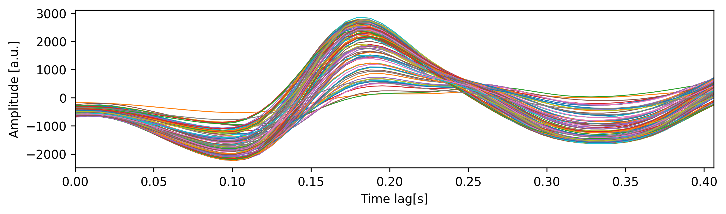
The TRF.plot() method allows a quick visualization of the weights after training theTRF. Because the weight matrix is three-dimensional (inputs-by-lags-by-outputs) visualization requires selecting from or averaging across one of the dimensions. In the below example, we are plotting the TRFs weights over time for the 7 ^th feature (i.e. spectral band) for each channel as well as the global field power (i.e. standard deviation across all channels) for every feature.

from matplotlib import pyplot as plt
fig, ax = plt.subplots(2)
fwd_trf.plot(feature=6, axes=ax[0], show=False)
fwd_trf.plot(channel='gfp', axes=ax[1], kind='image', show=False)
plt.tight_layout()
plt.show()

The top panel shows the forward TRFs weights across time. This is conceptually similar to an evoked response potential since the weights quantify the average effect a stimulus has on the neural response at a given delay. The bottom panel shows the color coded weights for each spectral band - bright yellow corresponds to high and dark blue to low weights. This depiction is also referred to as a spectrotemporal receptive field (STRF) because it shows the neural response to sound as a function of time and frequency.

It is not recommended to visualize a backward TRF in the same way. That is because the backward model must not only amplify the signal of interest (i.e. the neural activation pattern) but also suppress all signals of no interest. If those patterns are not orthogonal, the trade-off between amplification and suppression results in a complex spatial structure where the meaning of model weights can not be disentangled between the two tasks. However, we can transform backward to forward models [3] to allow a physiological interpretation of model weights:

transformed = bwd_trf.to_forward(response)
transformed.plot(feature=0)

Finally, we provide a method to easily convert a TRF to the MNE-Python framework. MNE is the most commonly used package for analyzing EEG and MEG data in Python and provides useful functions for visualization. The TRF.to_mne_evoked() requires information about channel locations (here, we use a standard montage for the biosemi system) and returns a list of mne.Evoked instances - one for each feature in the TRF. In the below example, we are converting and visualizing the TRF for the 7 ^th spectral band

from mne.channels import make_standard_montage

# use standard montage for the EEG system used for recording the response
montage = make_standard_montage('biosemi128')
evokeds = fwd_trf.to_mne_evoked(montage)
evokeds[6].plot_joint([0.11, 0.185, 0.29], topomap_args={"scalings": 1}, ts_args={"units": "a.u.", "scalings": dict(eeg=1)})

The scalp topographies show the spatial pattern of TRF weights at specific points in time which can be informative of the underlying neural generators.